Mastering the Confusion Matrix: Understand and Utilize this Powerful Evaluation Tool

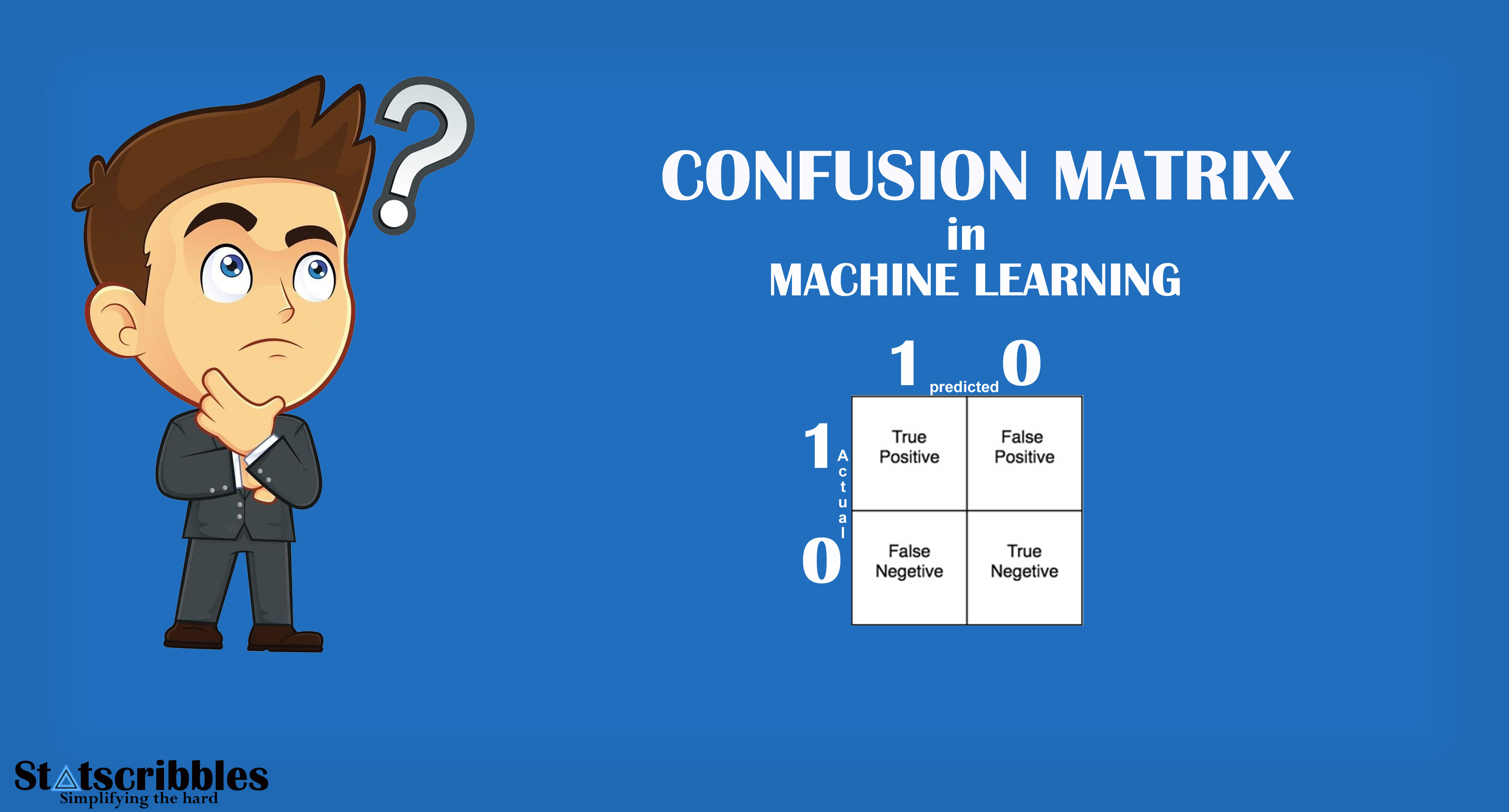
In simple terms, the Confusion matrix is an evaluation metric used to measure the performance of a machine learning model.

Let’s imagine that we have created a machine learning classification model that can identify whether an image is a dog’s image or a cat’s image. Now we need to know how many images have been correctly classified and how many have been incorrectly classified. The confusion matrix comes in handy to help us.

While classifying the images of Dogs and Cats there are four possibilities.

  • Correctly Identify Dog’s image
  • Correctly Identify Cat’s image
  • Incorrectly identify Dog’s image as Cat
  • Incorrectly identify Cat’s image as Dog

The four possibilities listed above are explained by the confusion matrix’s four main terms.

  • True Positive (TP)
  • True Negative (TN)
  • False Positive (FP)
  • False Negative (FN)

Let’s consider Dog’s image as a positive class and Cat’s image as a negative class.

True Positive

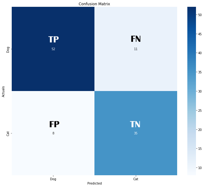
 When the actual image is Dog’s image and our classification model also predicts it correctly, it is True Positive. In other words, it has Truly identified the Positive class. In our above example, we have 52 True Positive cases.

True Negative

When the actual is Cat’s image and our classification model also predicts it correctly, it is True Negative. In other words, it has Truly identified the Negative class. In our above example, we have 35 True Negative cases.

False Positive (Type 1 error)

When the actual is Cat’s image, but our classification model predicts it as Dog, it is False Positive. That is, it has Falsely classified it to be a Positive class. In our above example, we have 8 cases of False Positive.

False Negative (Type 2 error)

When the actual is Dog’s image but our classification model predicts it as Cat, it is False Negative. In other words, the model has Falsely classified it to be a Negative class. In our above example, we have 11 cases of False Negative.

We can calculate other metrics like Accuracy, Precision, Recall, and F1-score using TP, TN, FP, and FN.
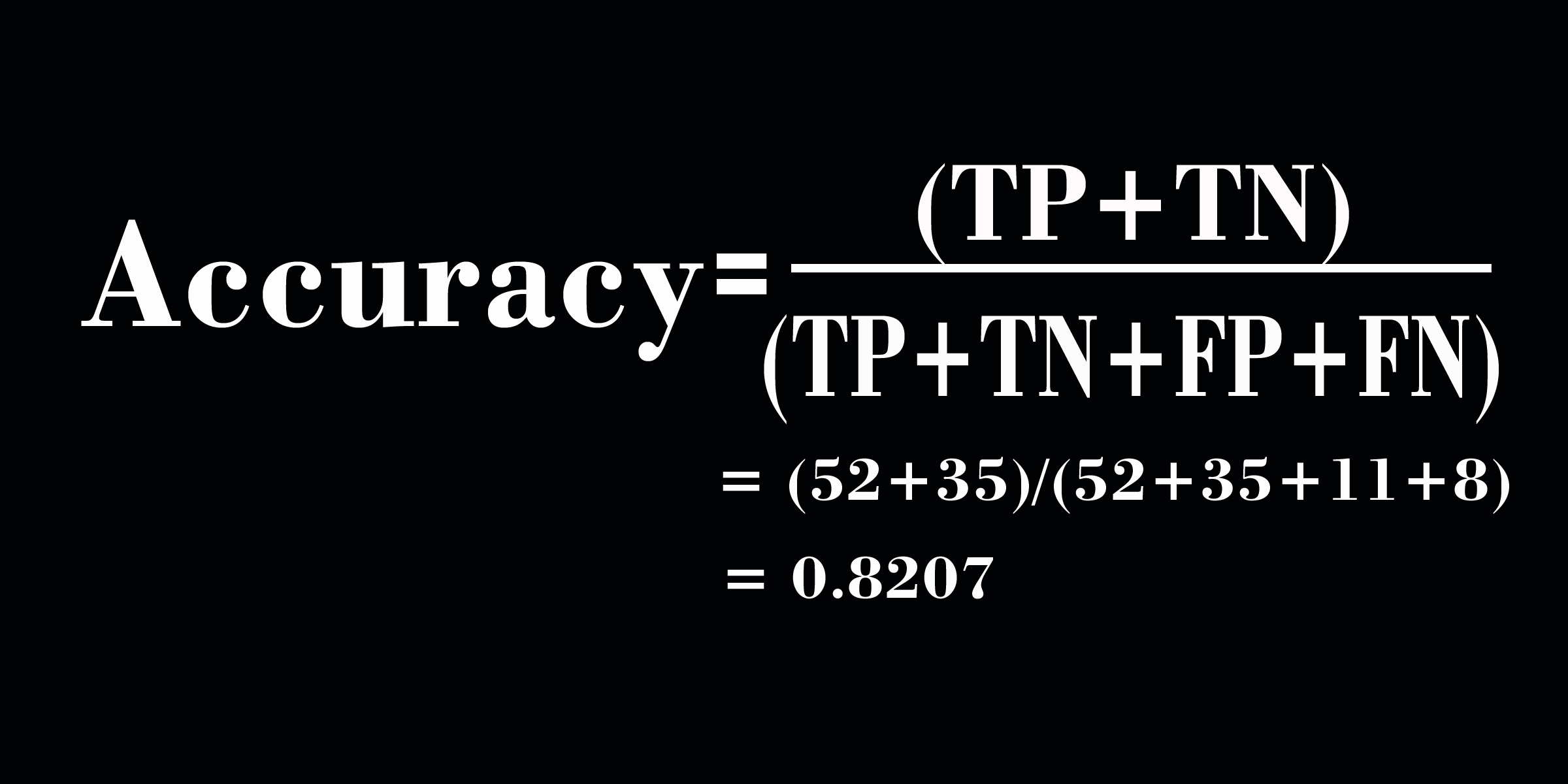
Accuracy

Accuracy measures, how correctly our model has predicted the positive and Negative classes. The formula’s numerator is TP+TN (Total number of classes correctly identified as Positive and Negative), and the denominator is TP+TN+FP+FN(All). Higher the Accuracy, the better our model. In particular, accuracy is not the best metric when your dataset is imbalanced.
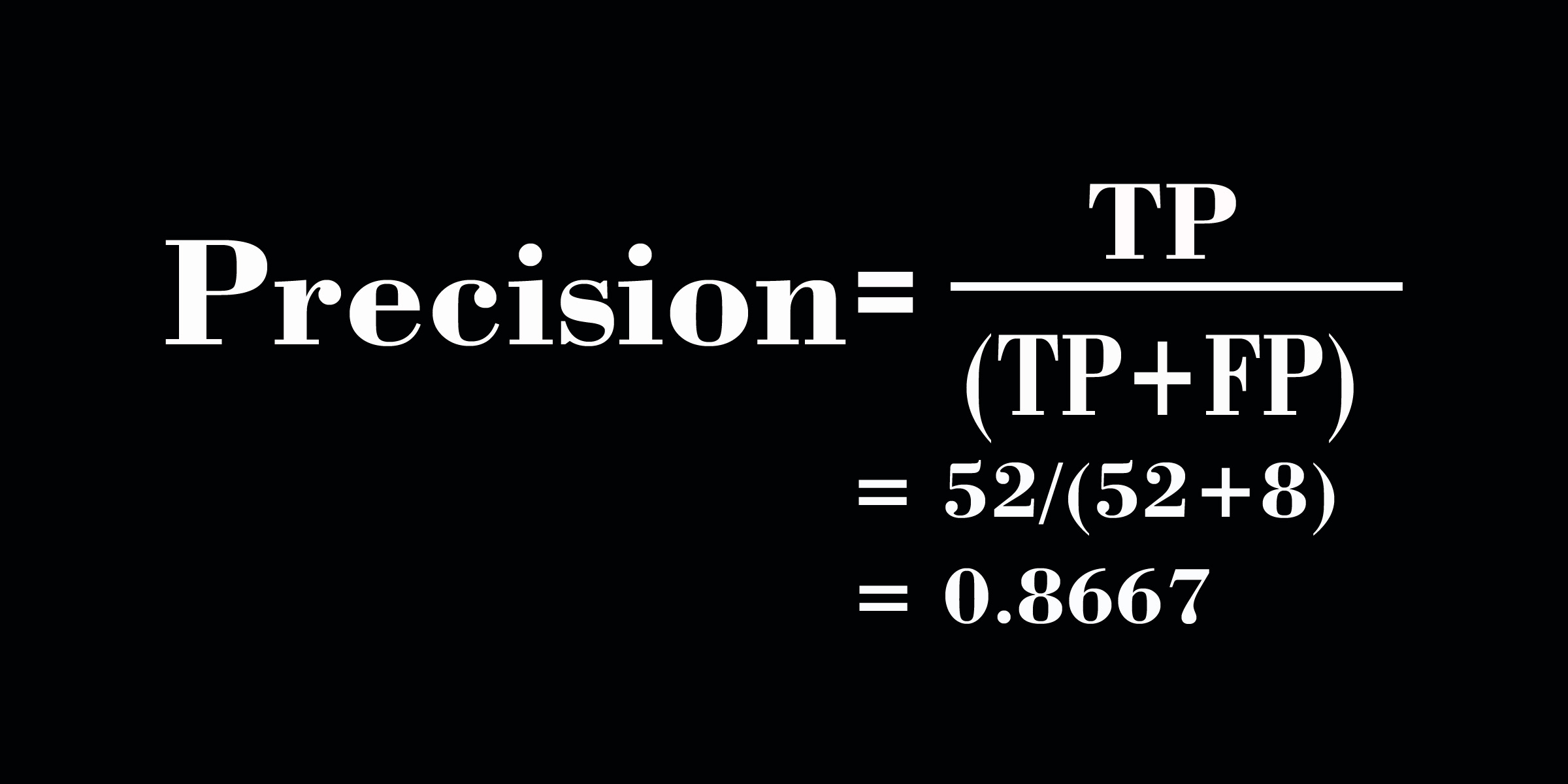
Precision

Precision measures, out of all Positive predictions, how many are truly positive? In the formula, the numerator is TP and the denominator is TP+FP. So if False positive cases increase, our precision score decreases, and vice versa. Hence If we aim to reduce the False Positive cases, then Precision becomes our optimal metric, and we need to focus on improving it.
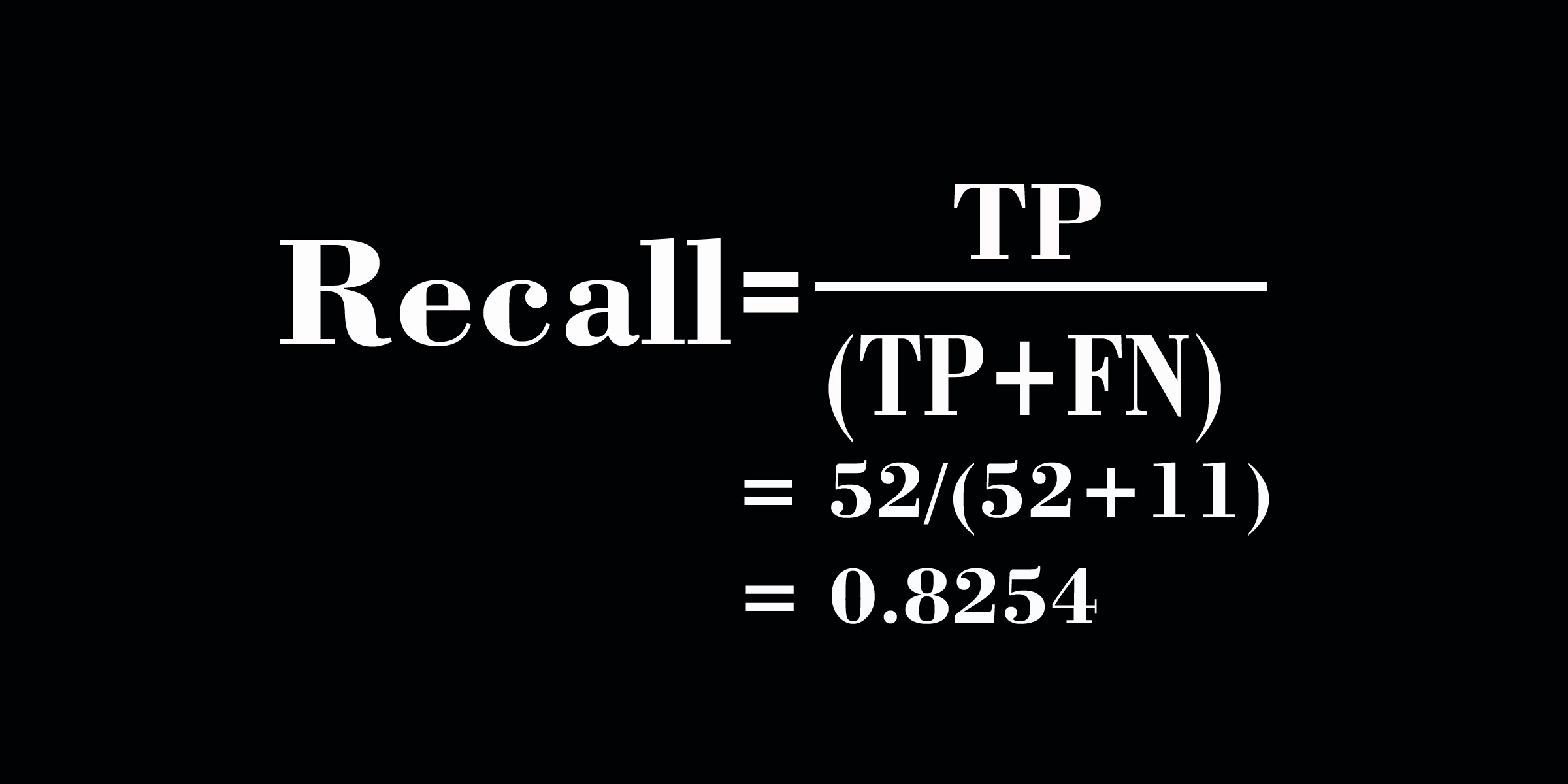
Recall

Recall measures, out of all Actual Positive cases, how many have been correctly identified as positive by our model? In the formula, the numerator is TP and the denominator is TP+FN. So if False Negative cases increase, our Recall score decreases, and vice versa. Hence If we aim to reduce False Negative cases, then Recall becomes our optimal metric, and we need to focus on improving it.

F1-Score

In our problem statement, if it is crucial to maintain both False Positive and False Negative rates, then the optimal metric is the F1-score. It takes the harmonic mean of Recall and Precision.

The main reason to take the harmonic mean instead of the simple average is that the simple average gives equal weightage to all the values involved in the calculation, while the harmonic mean gives more importance to the low value and penalizes the higher value.

For example, if precision is 0.3 and recall is 0.9, then our simple average would be 0.6, which means the model’s performance is good. But our precision score is very low, so we will have more False Positive cases. The harmonic mean is 0.45, which means the model’s performance is not that good. It took into account the low precision score we had.

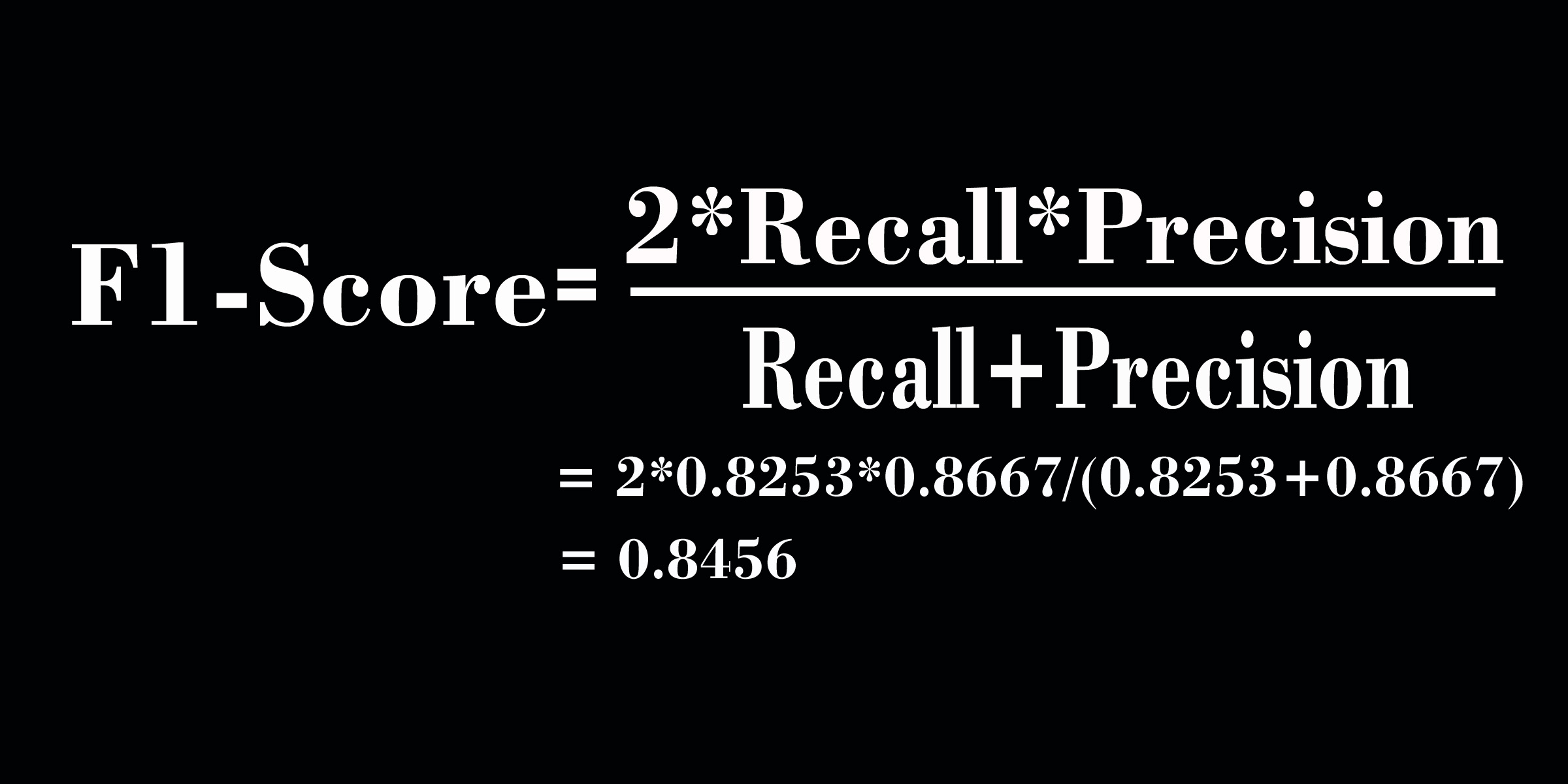
The more simplified version of F1-score formula will help us understand it more easily.

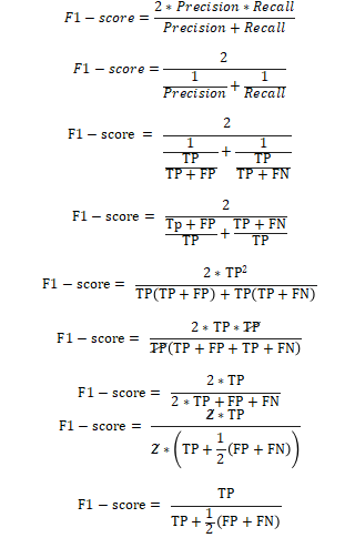
In the above formula, we can see that equal weight is given to both FP and FN, so the harmonic mean takes care of the extreme values of FP and FN. Hence F1-score becomes an optimal metric to have a balance between FP and FN.

Conclusion

I hope that this blog post helped you understand the Confusion matrix and the metrics that go along with it. Although we used a binary classification example, the Confusion matrix is so effective that we can also use it for problems involving multiple classes of classification.

SQL Queries – Order of Execution

Any aspirant data professional should be knowledgeable about the Order of Execution of SQL Queries because it is crucial in both interviews and the workplace. By allowing you to create effective queries and prevent unexpected outputs, it simplifies your life. As a data scientist, I attended interviews with numerous firms, and 2 out of 5 interviewers inquired about the SQL queries’ order of execution.

Order of execution in SQL

Although SQL may appear to be a simple language, as we dig deeper, we will understand how powerful it is. Its support for complex queries is simply incredible.. SQL queries mainly has following statements

  • Select
  • From
  • Join
  • Where
  • Group by
  • Having
  • Order by
  • Offset/Limit

With the following example we can understand the order of execution.

Let us consider 2 tables, a transaction table and product table.

Transaction Table Name : ‘transaction’

Product Table Name:  ‘Product’

The transaction table contains txn_id, prd_id, qty and msrp columns.
The product table contains prd_id and prd_cat columns.

FROM

The FROM statement, which identifies the table from which data is fetched, is the first statement to be run in a SQL query. The query in the example below has two problems: the table name is misspelled , and the column ’emp_id’ isn’t present in the transaction table. Still, we only receive the message that ‘statscribbles.statscribbles_db.transaction_1’ table cannot be located.

When I correct the table name  in below example we could see that SQL identifies the issue in column name specified. This demonstrates unequivocally that the first statement to be executed in a query is ‘FROM’.

JOIN CLAUSE

A Join clause will get executed second in the SQL Query ,it is used to combine rows from two or more tables based on the common columns between the tables. Even in the example below, I used the wrong column name in the join condition and in select statement. We could see  that SQL first identifies the incorrect column name in join condition rather than the column name in select statement. This demonstrates unequivocally that the ‘join’ statement is executed prior to the ‘select’ statement.

WHERE

The Where statement is the third to be run in a SQL query. By using the specified criteria, it is used to filter the output of the tables obtained from the “FROM” statement and join clause. In the below example also incorrect column in where condition is identified first rather than incorrect column name in select statement.

GROUP BY

The fourth statement to get executed in an SQL query is Group by clause. It is used to aggregate the data based on one or more columns. If the query contains a Where clause, Group by will run after the Where clause has filtered the data. Despite the fact that the select, where, and group by statements in the example below use wrong column names, SQL initially recognizes the error in the where condition.  This demonstrates unequivocally that Group by is executed only after where statement.

HAVING CLAUSE

The Having clause is the fifth statement that a SQL query executes. It is used to filter the data in the table similar to  Where clause, however the distinction is that the Where clause is executed before the Group by clause and the Having clause is executed after the Group by clause.When establishing a condition in a where clause, aggregate functions cannot be used; however, they may be used in a having clause. The below example clearly shows that aggregate functions cannot be used in where clause.

SELECT

The sixth statement to get executed in SQL query is select. In spite of being present at the very beginning Select statement is actually executed at sixth place. The above mentioned statements decides the records which has to be present in the result table where as Select statement specifies the columns that needs to be present in the result.

ORDER BY

The seventh statement to get executed in SQL query is Order by. Once the tables have been chosen ,necessary records and columns have been filtered using the statements mentioned above we can now order the result based on one or more columns using Order By clause. We can order the result either in Ascending or Descending order of specified columns.

Offset/Limit

The last statement to get executed is offset & limit statements with which we can retrieve a subset of data. In the below example we have taken  list of product category and number of products in that category provided that the ‘msrp’ of those products are  greater than 70.

From the above example, if we only wanted the product categories that have the second most number of products we can use offset and limit as mentioned in the query below. Offset 1 gets a subset of the table from row number 2 till the end and limit 1 gets only the first row from that subset.